Build a packing list from your Squarespace orders in Google Sheets

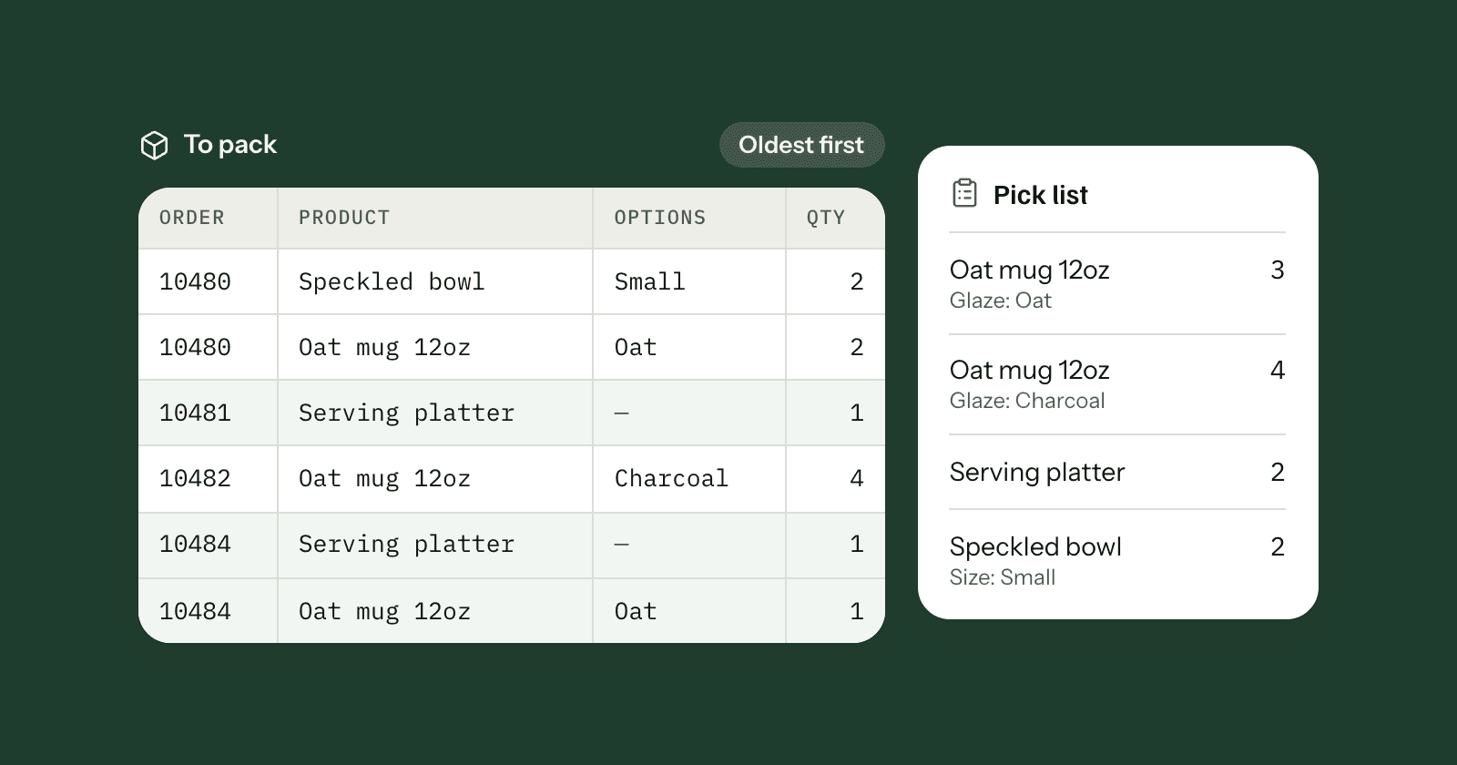
This guide is for makers and small shops who pack orders by hand and want one list to work from. By the end you'll have two new sheets in your Google Sheets spreadsheet: To pack, which lists the items of every order you haven't fulfilled yet, oldest order first, with options and product form answers; and Pick list, which adds up how many of each product and option you need to make or pull from the shelves. Both update on their own, and an order drops off the list once you mark it fulfilled in Squarespace.

How it works

SuperJack syncs your Squarespace orders into a sheet every hour. Each sync updates the whole order history, so the sheet always matches your store: new orders appear, and when you fulfill or cancel an order in Squarespace, its Fulfillment Status changes in the sheet too.

The packing list is a formula on its own sheet that reads from that synced sheet and keeps only the orders whose Fulfillment Status is PENDING. Squarespace uses three values for that field, PENDING, FULFILLED and CANCELED (Squarespace Orders API), so pending means "paid for, not shipped or handed over yet".

Keep your own work off the synced sheet. SuperJack keeps that sheet matching your store, so anything you type into it is replaced on the next sync. The formulas below go on new sheets (tabs) that read from it.

If you haven't connected your store yet, follow how to sync Squarespace orders to Google Sheets first. It takes about two minutes.

Before you start: three things to check

Open the spreadsheet SuperJack syncs to and look at the synced sheet.

1. Its name. The formulas below call it Orders. If yours is called something else, like Sheet1, change Orders in the formulas. Put quotes around names with spaces: 'Shop orders'!A1:AF1.
2. Its last column. The formulas use AF. Scroll right to the last column with a heading and change AF to that letter. Your sheet might be wider or narrower than ours, depending on your checkout and product form questions.
3. Where the headings are. Headings are on row 1, unless you turned on Show the last sync time in SuperJack. Then the sync time is in cell A1 and the headings move to row 2, so use Orders!A2:AF2 for the headings and Orders!A3:AF for the data.

The formulas find columns by their heading, like "Fulfillment Status" or "Quantity", not by letter. Hiding a column in SuperJack's column picker or adding a new form question won't break them. Just keep the columns they use switched on.

Step 1: the "To pack" sheet

1. Click + at the bottom left of Google Sheets to add a sheet, and name it To pack.
2. In row 1, type the headings: Order, First name, Last name, Product, Options, Qty, Product form.
3. Click cell A2 and paste this formula:

=LET(
  head, Orders!A1:AF1,
  data, Orders!A2:AF,
  status, INDEX(data, 0, MATCH("Fulfillment Status", head, 0)),
  rows, FILTER(data, status = "PENDING"),
  SORT({
    INDEX(rows, 0, MATCH("Order Number", head, 0)),
    INDEX(rows, 0, MATCH("BA - First Name", head, 0)),
    INDEX(rows, 0, MATCH("BA - Last Name", head, 0)),
    INDEX(rows, 0, MATCH("Name", head, 0)),
    INDEX(rows, 0, MATCH("Options", head, 0)),
    INDEX(rows, 0, MATCH("Quantity", head, 0)),
    INDEX(rows, 0, MATCH("Product Custom Form", head, 0))
  }, 1, TRUE)
)

Here's what it does, line by line:

• head and data are the synced sheet's headings and its rows.
• status is the Fulfillment Status column, found by its heading.
• rows keeps only the rows where the status is PENDING.
• The { ... } block picks the columns for your list, each found by heading, and SORT(..., 1, TRUE) sorts by order number, smallest first. Squarespace order numbers go up with every order, so that's oldest first, whichever way round SuperJack's Oldest orders first option is set.

SuperJack writes one row per item, like Squarespace's own CSV export, so an order with three products takes three rows. Sorted by order number, those rows sit together, which groups each order for you.

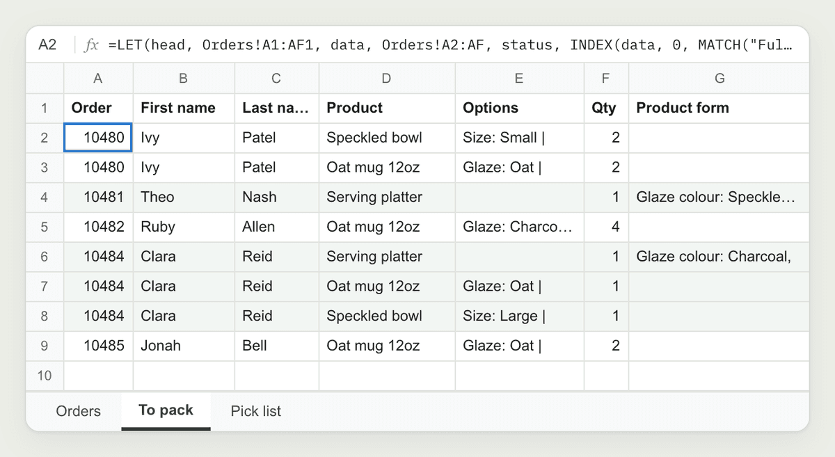
Add a column for any form answer. Every checkout form question gets its own column in the synced sheet, named Checkout Form: followed by the question. To show a gift note, add a heading in column H and this line to the { ... } block, after the Product Custom Form line (put a comma after that line first):

INDEX(rows, 0, MATCH("Checkout Form: Gift note", head, 0))

Use the heading exactly as it appears in your synced sheet. There's more on these columns in getting Squarespace custom form answers into Google Sheets.

When everything is packed, the formula shows #N/A with "No matches are found in FILTER evaluation". That's the good news: nothing is pending.

Optional: shade every other order

To make each order easier to see at a glance:

1. Select columns A to G from row 2 down (click A2, then Shift-click the last row you need in column G).
2. Click Format > Conditional formatting.
3. Under Format rules, choose Custom formula is and enter:

=AND($A2 <> "", ISEVEN(COUNTUNIQUE($A$2:$A2)))

4. Pick a light fill colour and click Done.

The formula counts how many different order numbers there are down to each row, and shades the rows of every second order.

Step 2: the "Pick list" sheet

The pick list answers a different question: across everything still to pack, how many of each product and option do you need? Add a sheet called Pick list and paste this into cell A1. It writes its own headings.

=LET(
  head, Orders!A1:AF1,
  data, Orders!A2:AF,
  QUERY({
    INDEX(data, 0, MATCH("Name", head, 0)),
    INDEX(data, 0, MATCH("Options", head, 0)),
    INDEX(data, 0, MATCH("Quantity", head, 0)),
    INDEX(data, 0, MATCH("Fulfillment Status", head, 0))
  }, "select Col1, Col2, sum(Col3) where Col4 = 'PENDING' group by Col1, Col2 order by sum(Col3) desc, Col1 label Col1 'Product', Col2 'Options', sum(Col3) 'To make'", 0)
)

The { ... } block builds a small table of product name, options, quantity and status. QUERY then keeps the pending rows, groups them by product and option, and adds up the quantities, biggest first. Inside QUERY, Col1 to Col4 are the four columns of that small table, so no letters from your synced sheet are involved.

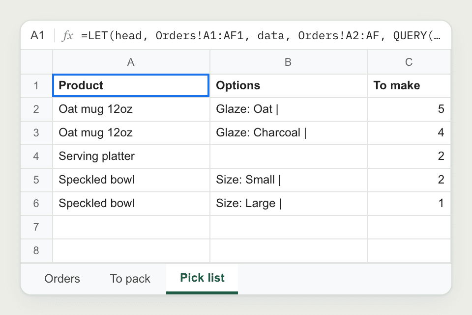
The Options column shows variants the way SuperJack writes them, for example Glaze: Oat |. Products without variants have an empty Options cell and are added up together.

Why not a checkbox column?

It's tempting to add a "Packed" checkbox next to the To pack list. We'd advise against it. The list is a formula result, so its rows move whenever an order is added, fulfilled or cancelled. A checkbox you typed in row 5 stays in row 5 while the order beside it moves, and soon the ticks sit next to the wrong orders.

Instead, mark the order fulfilled in Squarespace when it's packed. That's where your customer gets their shipping email anyway. On the next hourly sync the order's status changes to FULFILLED and it drops off both sheets. If you want it gone sooner, open the workflow in SuperJack and click Run a test sync.

Print it for the packing table

1. Open the To pack sheet (or Pick list).
2. Click File > Print.
3. Under Print, choose Current sheet.
4. Set Page orientation to Landscape and Scale to Fit to width, so every column fits on the page.
5. Click Next and print, or save as a PDF.

If you only want part of the list, select those rows first and choose Selected cells instead of Current sheet.

A note on commas and semicolons

If your spreadsheet's locale uses a comma as the decimal point (most of Europe, for example), Google Sheets separates formula arguments with semicolons and the columns inside { ... } with backslashes. Swap them in when you paste, or set File > Settings > Locale to United States.

What to build next

The same pattern works for any view of your orders: track your stock levels next to what's selling, or build sales reports by month.

SuperJack syncs your Squarespace orders to Google Sheets every hour, custom form answers included. Start your free trial: you get 3 days to try it, and you can cancel any time.