Squarespace sales reports in Google Sheets: revenue by month and best sellers

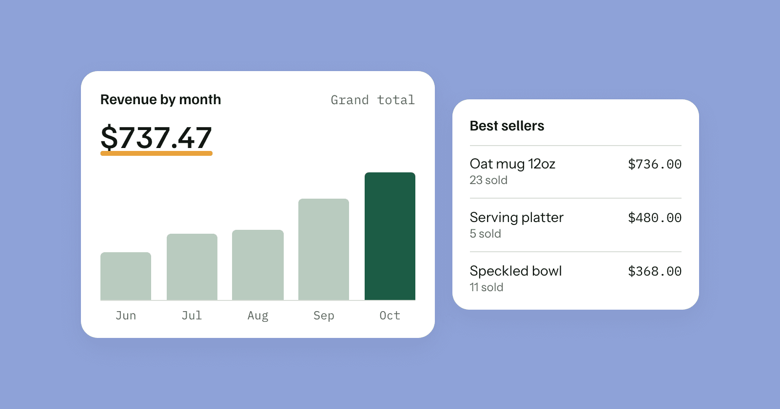
This guide is for Squarespace store owners who want to answer "how did we do this month?" and "what sells best?" from their own spreadsheet. By the end you'll have revenue by month with a chart, a best sellers list by units and revenue, your refunds, and how often each promo code was used. Everything reads from the orders sheet SuperJack keeps up to date, so the reports update themselves every hour.

If your orders aren't in Google Sheets yet, start with how to sync Squarespace orders to Google Sheets.

First, the one thing that trips everyone up

SuperJack writes one row per item ordered, like Squarespace's own CSV export. An order with three products takes three rows, and the order's details are repeated on each one: Order Number, Created On, Subtotal, Grand Total, Refunded Total, Promo Codes and so on.

That's what you want for product reports, but it means you can't add up the Grand Total column. Order 10484 in our sample store has three items, so its $173.35 appears three times. Adding up the whole column gives $2,524.56, while the real total of those orders is $1,729.30.

So there are two kinds of numbers, and each needs its own method:

• Order totals: Grand Total, Subtotal, Refunded Total. These belong to the order, so count each order once. Grand Total is what the customer paid, including shipping and tax.
• Item revenue: Price × Quantity on each row. Price is the price paid for one unit, so this adds up product sales and leaves out shipping and tax. Use it to compare products.

The two won't match, and that's expected. In the sample store, item revenue is $1,584.00 against $1,729.30 in order totals; the difference is shipping and tax, less discounts.

Keep your reports on their own sheets (tabs). SuperJack keeps the synced sheet matching your store, so anything you type into it is replaced on the next sync. Each sync updates the whole order history, which is also why refunds and cancellations show up in your reports without you doing anything.

Before you start

The formulas call the synced sheet Orders and its last column AF. Change both to match your sheet: the name on its tab, and the letter of the last column with a heading. Put quotes around names with spaces, like 'Shop orders'!A1:AF1. If Show the last sync time is on in SuperJack, headings are on row 2, so use Orders!A2:AF2 and Orders!A3:AF.

The formulas find columns by their heading, not their letter, so switching columns off in SuperJack or adding form questions won't break them.

Step 1: one row per order

1. Add a sheet with + at the bottom left and name it Order totals.
2. In row 1, type the headings: Order, Created On, Subtotal, Grand Total, Refunded, Status, Promo code.
3. In A2, paste:

=LET(
  head, Orders!A1:AF1,
  data, Orders!A2:AF,
  num, INDEX(data, 0, MATCH("Order Number", head, 0)),
  UNIQUE(FILTER({
    num,
    INDEX(data, 0, MATCH("Created On", head, 0)),
    INDEX(data, 0, MATCH("Subtotal", head, 0)),
    INDEX(data, 0, MATCH("Grand Total", head, 0)),
    INDEX(data, 0, MATCH("Refunded Total", head, 0)),
    INDEX(data, 0, MATCH("Fulfillment Status", head, 0)),
    INDEX(data, 0, MATCH("Promo Codes", head, 0))
  }, num <> ""))
)

It picks only order-level columns. Those are identical on every row of the same order, so UNIQUE keeps one row per order. The FILTER drops the empty rows below your data.

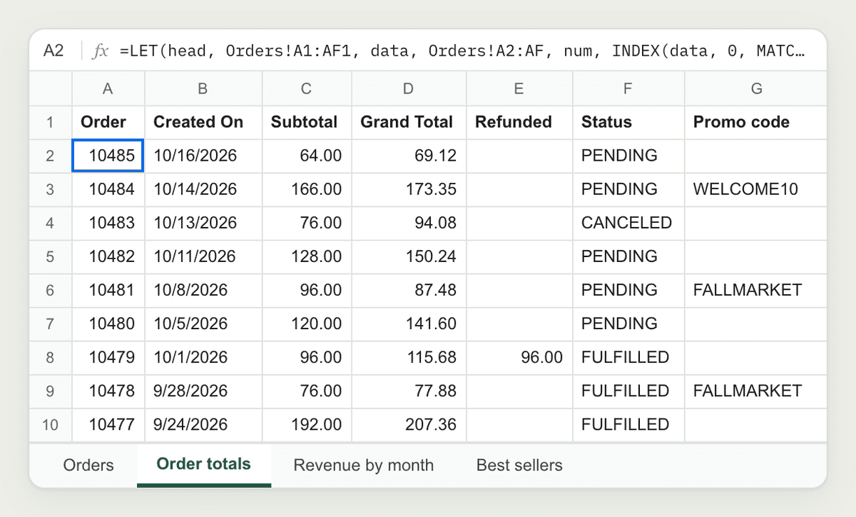
If the Created On column shows numbers like 46311.3, select column B and choose Format > Number > Date time.

Check that dates are dates. Monthly reports need Google Sheets to read Created On as a date. SuperJack writes it as month/day/year in your store's time zone, for example 10/16/2026 8:03:00 AM, which a spreadsheet set to a month-first locale such as United States reads as a date and time. To check, type =ISNUMBER('Order totals'!B2) in an empty cell. If it says FALSE, go to File > Settings, set Locale to United States and click Save settings. Each sync updates the whole order history, so after the next sync (or Run a test sync in SuperJack) the dates are read as dates.

Step 2: revenue by month, with a pivot table

A pivot table groups and adds up rows for you, and works straight from headings.

1. On the Order totals sheet, click the column letter A, then Shift-click G to select columns A to G.
2. Click Insert > Pivot table, choose New sheet and click Create. Rename the new sheet Revenue by month.
3. In the pivot table editor, next to Rows, click Add and choose Created On.
4. Next to Values, click Add and choose Order, then change Summarize by to COUNTA. That counts orders.
5. Add Grand Total and Refunded to Values too, summarized by SUM.
6. Next to Filters, click Add and choose Status. Under Status, click the drop-down, untick CANCELED (and (Blanks) if it's there) and click OK.
7. In the pivot table, right-click any date under Created On and choose Create pivot date group > Year-Month.

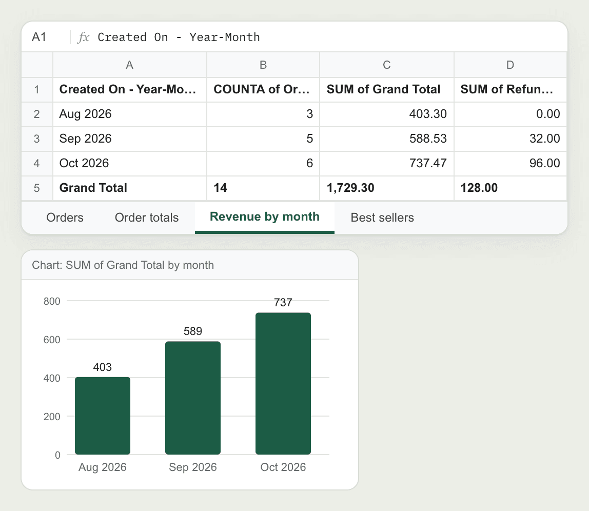
You now have one row per month, with the number of orders, the revenue and the refunds.

Add a chart

1. Click any cell in the pivot table.
2. Click Insert > Chart.
3. In the chart editor, under Chart type, choose Column chart.
4. Under Series, remove the ones you don't want to plot, such as COUNTA of Order, so the chart shows revenue by month.

The chart follows the pivot table, so it grows a new column each month.

Step 3: best sellers by units and revenue

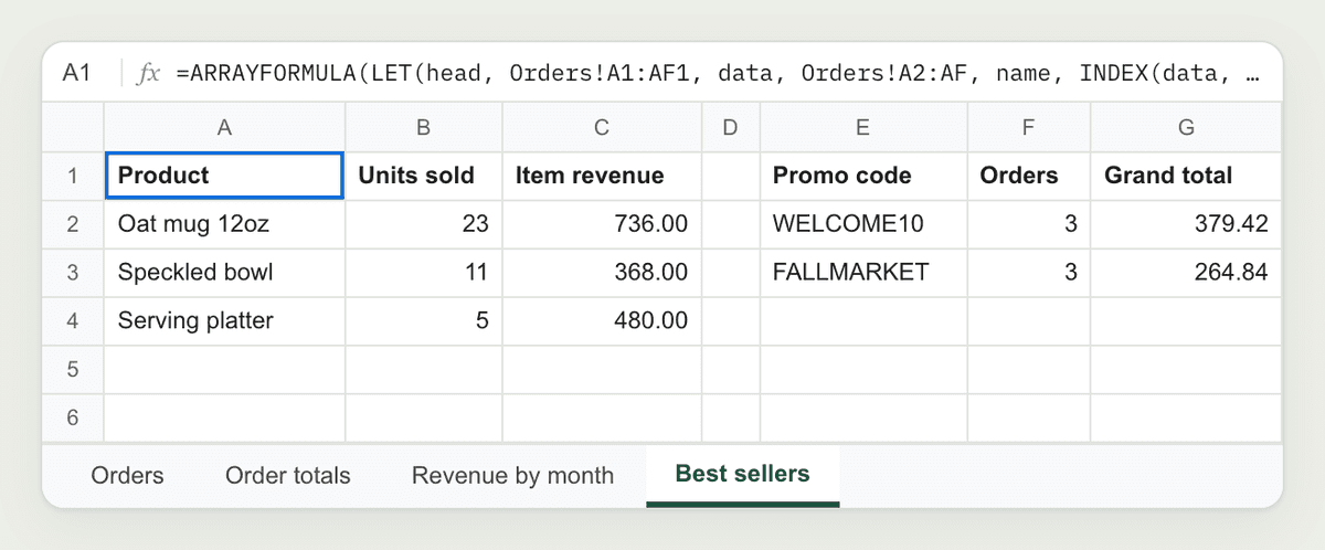
For product numbers, go back to the item rows. Add a sheet called Best sellers and paste this into A1. It writes its own headings.

=ARRAYFORMULA(LET(
  head, Orders!A1:AF1,
  data, Orders!A2:AF,
  name, INDEX(data, 0, MATCH("Name", head, 0)),
  qty, INDEX(data, 0, MATCH("Quantity", head, 0)),
  price, INDEX(data, 0, MATCH("Price", head, 0)),
  status, INDEX(data, 0, MATCH("Fulfillment Status", head, 0)),
  QUERY({name, qty, price * qty, status}, "select Col1, sum(Col2), sum(Col3) where Col1 is not null and Col4 <> 'CANCELED' group by Col1 order by sum(Col2) desc label Col1 'Product', sum(Col2) 'Units sold', sum(Col3) 'Item revenue'", 0)
))

The { ... } block builds a small table of product, quantity, price × quantity and status. ARRAYFORMULA makes the multiplication work on every row at once. QUERY then leaves out cancelled orders, groups by product and adds up units and item revenue, most units first. To rank by revenue instead, change order by sum(Col2) desc to order by sum(Col3) desc.

Refunds

Refunded Total is an order-level field, so use the Order totals sheet. Squarespace reports refunds in their own field, and the cell is empty when nothing was refunded. In any empty cell:

=SUM('Order totals'!E2:E)

=COUNTIF('Order totals'!E2:E, ">0")

The pivot table in step 2 already shows refunds by month.

Promo code usage

Promo codes belong to the order too. On the Best sellers sheet, paste this into E1, leaving a gap column after the best sellers list:

=QUERY('Order totals'!A2:G, "select G, count(A), sum(D) where G is not null and F <> 'CANCELED' group by G order by count(A) desc label G 'Promo code', count(A) 'Orders', sum(D) 'Grand total'", 0)

This one can use column letters, because you set the columns of Order totals yourself in step 1: G is the promo code, A the order, D the Grand Total and F the status. Promotions applied without a code show under their name. An order that used two codes shows them together, like WELCOME10, FALLMARKET, and is counted under that pair.

If your formulas show an error

• #N/A saying MATCH couldn't find a value: a heading is spelled differently or switched off in SuperJack's column picker. Check the synced sheet's headings.
• #REF! saying the array result was not expanded: something is typed in the cells below or beside the formula that its result needs. Empty those cells.
• Formulas show as errors right after pasting: if your locale uses a comma as the decimal point, Google Sheets uses semicolons between arguments and backslashes between columns inside { ... }. Swap them in, or set the locale to United States.

What to build next

The same orders sheet can drive a packing list of unfulfilled orders, and with a products workflow, a low stock list.

SuperJack syncs your Squarespace orders to Google Sheets every hour, custom form answers included. Start your free trial: you get 3 days to try it, and you can cancel any time.